Analysis of the margin width in a soft-margin SVM

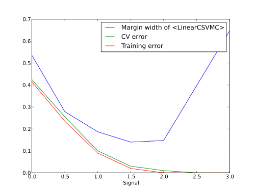
Width of the margin of soft-margin SVM (mvpa2.clfs.svm.LinearCSVMC) is not monotonic in its relation with SNR of the data. In case of not perfectly separable classes margin would first shrink with the increase of SNR, and then start to expand again after learning error becomes sufficiently small.

This brief examples provides a demonstration.

import mvpa2
import pylab as pl
import numpy as np
from mvpa2.misc.data_generators import normal_feature_dataset
from mvpa2.clfs.svm import LinearCSVMC
from mvpa2.generators.partition import NFoldPartitioner
from mvpa2.measures.base import CrossValidation
from mvpa2.mappers.zscore import zscore

Generate a binary dataset without any signal (snr=0).

mvpa2.seed(1);
ds_noise = normal_feature_dataset(perlabel=100, nlabels=2, nfeatures=2, snr=0,
                                  nonbogus_features=[0,1])

# signal levels
sigs = [0, 0.5, 1.0, 1.5, 2.0, 2.5, 3.0]

To mimic behavior of hard-margin SVM whenever classes become separable, which is easier to comprehend, we are intentionally setting very high C value.

clf = LinearCSVMC(C=1000, enable_ca=['training_stats'])
cve = CrossValidation(clf, NFoldPartitioner(), enable_ca='stats')
sana = clf.get_sensitivity_analyzer(postproc=None)

rs = []
errors, training_errors = [], []

for sig in sigs:
    ds = ds_noise.copy()
    # introduce signal into the first feature
    ds.samples[ds.T == 'L1', 0] += sig

    error = np.mean(cve(ds))
    sa = sana(ds)
    training_error = 1-clf.ca.training_stats.stats['ACC']

    errors.append(error)
    training_errors.append(training_error)

    w = sa.samples[0]
    b = np.asscalar(sa.sa.biases)
    # width each way
    r = 1./np.linalg.norm(w)

    msg = "SIGNAL: %.2f training_error: %.2f error: %.2f |w|: %.2f r=%.2f" \
      %(sig, training_error, error, np.linalg.norm(w), r)
    print msg

    # Drawing current data and SVM hyperplane+margin
    xmin = np.min(ds[:,0], axis=0)
    xmax = np.max(ds[:,0], axis=0)
    x = np.linspace(xmin, xmax, 20)
    y  =    -(w[0] * x - b) /w[1]
    y1 = ( 1-(w[0] * x - b))/w[1]
    y2 = (-1-(w[0] * x - b))/w[1]

    pl.figure(figsize=(10,4))

    for t,c in zip(ds.UT, ['r', 'b']):
        ds_ = ds[ds.T == t]
        pl.scatter(ds_[:, 0], ds_[:, 1], c=c)
    # draw the hyperplane
    pl.plot(x, y)
    pl.plot(x, y1, '--')
    pl.plot(x, y2, '--')
    pl.title(msg)
    ca = pl.gca()
    ca.set_xlim((-2, 4))
    ca.set_ylim((-1.2, 1.2))
    pl.show()
    rs.append(r)

So what would be our dependence between signal level and errors/width of the margin?

pl.figure()
pl.plot(sigs, rs, label="Margin width of %s" % clf)
pl.plot(sigs, errors, label="CV error")
pl.plot(sigs, training_errors, label="Training error")
pl.xlabel("Signal")
pl.legend()
pl.show()

And this is how it looks like.

See also

The full source code of this example is included in the PyMVPA source distribution (doc/examples/svm_margin.py).